Kinetic Model of Monoterpenoid Biosynthesis Wiki

In this study, the main aim is to gain insight and understanding on the production of various monoterpenoids such as limonene and mint, and to design strategies that could assist in improving the production of these terpenes. Therefore, mathematical models of enzymatic reactions and metabolic pathways in the engineered terpene synthesis network, as well as core primary metabolic pathways that supports this network are constructed. Ensemble modelling has been adopted as the modelling approach for these ODE-based models.

Ensemble modelling approach uses Bayesian statistics where we define a prior - an initial belief of what the kinetic parameter values for the reactions are - which is used for simulations that would result in a posterior that would inform the modeller of how well the kinetic value in describing the network or how well does the model(s) closely resembles the experimental observation. These predictions will drive to improve the model(s) by updating our prior.

As the models are ODE-based with kinetic parameters, common problem modellers face is the challenge to obtain the kinetic parameter values. These information are often scarce, if not incomplete or none at all.

This study models the engineered monoterpene synthesis network based on all known kinetic values for each of its reaction. The general modelling approach is a modular one where each of the enzymatic reaction in the network represents an individual model and can be imagined as individual lego bricks. These lego bricks can be assembled or disassembled according to our modelling objective- either to model an individual reaction or to model a specific set of reactions to mimic our engineered constructs. Each of the enzymatic reaction is described using reversible Michaelis-Menten equation which requires various kinetic parameters such as the Michaelis-Menten constant, the turnover number and the equilibrium constant. The values for these kinetic parameters are extensively sought from published reports, enzyme and metabolic databases such as BRENDA, UniProt, ENZYME and MetaCyc, as well as from experimentally measured enzymatic assays carried out within our group. Uncertainties within the kinetic values measured from varied sources are acknowledged and is included in the modelling process. This includes incorporating generic parameter values from the BRENDA database. Our initial belief of the uncertainties associated with each kinetic parameter is represented with a lognormal probability distribution, which provides a number of plausible values to be sampled during an ensemble modelling technique. More information on uncertainty and ensemble modelling adopted for this study can be found here.

Pathway models

The engineered monoterpene network and its enzymatic reactions

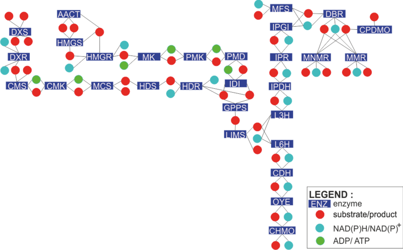
To find out how each enzyme in the network is modelled, click on the rectangles in the figure on the left. Alternatively, you can click the enzyme names from the list below.

IPP and DMAPP Biosynthesis Diphosphomelvalonate decarboxylase (DMD) Hydroxymethylbutenyl diphosphate reductase (HMBPPR) Limonene Biosynthesis Geranyl diphosphate synthase (GPPS) Limonene Synthase Peppermint Biosynthesis Limonene-3-hydroxylase (L3H) Isopiperitenol Dehydrogenase (IPDH) Isopiperitenol Reductase (IPR) Isopulegone Isomerase (IPGI)

Mint Biosynthesis Pulegone Reductase (PGR) DBR Menthone:Neomenthol reductase (MNMR) Menthone:Menthol reductase (MMR) Spearmint Biosynthesis Limonene-6-Hydroxylase (L6H) Carveol Dehydrogenase (CDH) OYE CHMO Methanofuran Biosynthesis Menthofuran synthase (MFS)

Rate laws used in the model

Reactions in these models are described reversibly using Michaelis-Menten rate law and Convenience kinetics

Michaelis-Menten rate law

In these models, the reversible Micahelis-Menten rate equation is used with a Haldane substitution to take into account thermodynamic consistency in the form of the equilibrium constant K_eq.

Reversible Uni-uni Michaelis-Menten rate law

This rate equation is used to describe reactions with one substrate and one product. The general form of this rate equation is shown as:

$v_\mathrm{reaction} = [Enz] * K_\mathrm{cat} * \cfrac {\cfrac{[S]}{Km_\mathrm{substrate}} * \left ( 1 - \cfrac {[P]}{[S]*K_\mathrm{eq}} \right )} {1 + \cfrac {[S]}{Km_\mathrm{substrate}} + \cfrac {[P]}{Km_\mathrm{product}}}$

where [Enz] is the enzyme concentratuion, and [S] and [P] corresponds to the concentration of the substrate and product respectively.

Convenience kinetics

Convenience kinetics is a generalised form of Michaelis-Menten kinetics that covers all possible stoichiometries, and describes enzyme regulation by activators and inhibitors . For this reason, convenience kinetics is used to describe reactions with more than two reactants.

For a reaction

$A_1 + A_2 + ... <-> B_1 + B_2 + ...$

with concentrations [A₁], [A₂], [A_i],[B₁], [B₂] and [B_i] the general form of convenience kinetics is as follows:

Failed to parse (PNG conversion failed; check for correct installation of latex and dvipng (or dvips + gs + convert)): v\left( a,b \right) = Enzyme * \cfrac {kcat_{forward} \prod_{i} ã_i - kcat_{reverse} \prod_{j} b˜_j}{\prod_{i} (1 + ã_i) + \prod_{j} (1 + b˜_j)-1}

where variables with atilde denote the normalised reactant concentrations ã_i = [A_i] /K_mA and b˜_i = [B_i] /K_mB

Kinetic Parameters

Strategies for Estimating Kinetic Parameter Values

Using Equilibrium Constant (K_eq) in the reversible Michaelis-Menten equation

Using the equilibrium constant in the reversible Michaelis-Menten reaction reduces the need to obtain or estimate Vmax_reverse parameter value, which is often not available in literature.

Using the Haldane relationship, the equilibrium constant (K_eq) can be written as:

${\color{Red}K_\mathrm{eq}} = [Enz]* \frac{Kcat_\mathrm{forward} * Km_\mathrm{product} }{Kcat_\mathrm{reverse} * Km_\mathrm{substrate}}$

Calculating the Equilibrium Constant (K_eq)

The equilibrium constant can be calculated from the ratio of the forward and reverse reaction rates as described in the above section, given that the values for these rates are known. Unfortunately, the information for these values are often difficult to find, especially for reverse reaction rates (Vmax_reverse).

As an alternative, the equlibrium constant, K_eq, can also be calculated from the Gibbs free energy of a reaction, ΔG_r, using the Van't Hoff isotherm equation:

$-ΔG^° = -RT ln K$

and by dividing both sides of the equation with RT, and later take the exponents of both sides, the K_eq can be calculated by this equation:

$K_\mathrm{eq} = exp \left ( \cfrac {-ΔG^{°'}}{RT} \right )$

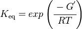
where;

Keq	Equilibrium constant
-ΔG°	Gibbs free energy change
R	Gas constant with a value of 8.31 JK-1mol-1
T	Temperature which is always expressed in kelvin

List of kinetic parameter values

Lists of values retrieved from published and unpublished sources for the kinetics of all the enzymes included in this study can be found here.

Abbreviations

List of abbreviations used in this study can be found here

Back to the main model page.

References

- ↑ Liebermeister, W. & Klipp, E. 2006. Bringing metabolic networks to life: convenience rate law and thermodynamics constraints.Theoretical Biology and Medical Modelling 3:41