Kinetic model of Central Metabolism
A kinetic model of glycolysis with serine activation is constructed from the literature data [1][2][3][4][5].
Contents
Description of the model
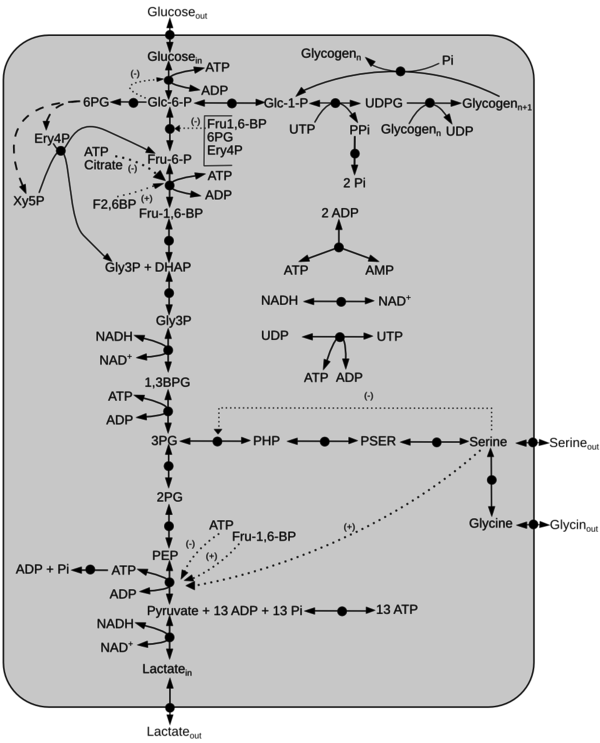
Schematic diagram of the model is given here. The dotted line represents activation(+) or inhibition(-) and the dashed arrow indicate Pentose Phosphate Pathway reactions not included in the model. Click on a reaction to have more information

Reactions
Details of the abbreviations for this model is listed here. Reactions of the model are listed below.
Initial concentration of the metabolites can be found here
Model File
The SBML file of the model can be found here
Notes
Necessary observation during model building and simulation is noted here.
Global parameters
Calculating 
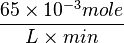
Some of the Vmax value in the paper "Modeling cancer glycolysis" is given in  unit [1]. To homogenize the units it is then converted back to
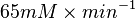
  by multiplying with 65 as the HeLa cell was incubated in
  .
.
- Converting to
 :
:

Also, 
We want to convert 1 to where HeLa cell was incubated in
Therefore, 
=> 
Striking out the necessary elements we get
=> 
Quantifying the flux
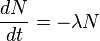
We used the Kinetic Flux Profiling (KFP) [6] method to quantify the flux values. The central idea of KFP is that larger metabolic fluxes cause faster transmission of isotopic label from added nutrient to downstream metabolites. Under pseudosteady state, if an external nutrient is instantaneously switched from natural to isotopically labeled, for a metabolite X directly downstream of nutrient assimilation, unlabeled  will be replaced over time by its labeled counterpart (
 ) and the fraction of unlabeled
  will decay. The rate constant of this decay
  is determined by the ratio of the flux through
  to the total pool size of
  .
.
- We used first order rate constant because, labeling decay is an exponential decay and the exponential decay follows first order rate constant.
and for first order rate equation
![- \frac{d[A]}{dt} = k[A]](/wiki/images/math/e/8/0/e802dbfb8a252f2bf0c9729a4e6e66bb.png)
- For exponential decay the slope is the height of the function.
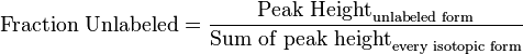
- First we determine the unlabeled from for each metabolites
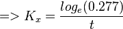
- If we can calculate the apparent first order rate constant
 then the flux can be calculated as
 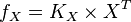 [
[ is the intracellular concentration of X ].
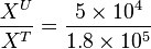
- With at steady-state, we calculate the change of unlabeled fraction with the introduction of label as
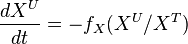
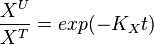
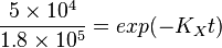
The analytical solution is
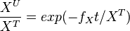
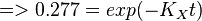
setting  , we get
Example:
To explain the procedure we took the example of Pyruvate in the presence of Serine and Glycine.
So,
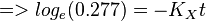
Now we know, . The intracellular concentration of  .
.
So, 
References
- ↑ 1.0 1.1 Marín-Hernández A, Gallardo-Pérez JC, Rodríguez-Enríquez S et al (2011). Modeling cancer glycolysis. Biochim Biophys Acta, 1807:755–767 (doi)
- ↑ Turnaev II, Ibragimova SS, Usuda Y et al (2006). Mathematical modeling of serine and glycine synthesis regulation in Escherichia coli. Proceedings of the fifth international conference on bioinformatics of genome regulation and structure 2:78–83
- ↑ Smallbone K, Stanford NJ (2013). Kinetic modeling of metabolic pathways: Application to serine biosynthesis. In: Systems Metabolic Engineering, Humana Press. pp. 113–121
- ↑ Palm, D.C. (2013). The regulatory design of glycogen metabolism in mammalian skeletal muscle (Ph.D.). University of Stellenbosch
- ↑ Ettore Murabito (2010). Application of differential metabolic control analysis to identify new targets in cancer treatment (Ph.D.). University of Manchester
- ↑ Yuan, J., Bennett, B.D. & Rabinowitz, J.D. (2008) Kinetic flux profiling for quantitation of cellular metabolic fluxes. Nat. Protoc. 3, 1328–1340