Kinetic Model of Monoterpenoid Biosynthesis Wiki

In this study, metabolic modelling is used to gain insight and understanding on the production of various monoterpenoids such as limonene and mint. We also aim to design strategies that could assist in improving the production of these terpenes. Here we present ODE-based models of the pathways in the engineered monoterpene synthesis network, as well as the supporting core primary metabolic pathways. These models are simulated and analysed using an ensemble modelling approach.

The ensemble modelling approach is based on the Monte-Carlo sampling method with Bayesian statistics. The approach defines a prior - an initial belief of what the kinetic parameter values for the reactions are - which is used for simulations that would result in a posterior that would inform the modeller of how well the kinetic value in describing the network or how well does the model(s) closely resembles the experimental observation. These predictions will drive to improve the model(s) by updating our prior.

As the models are ODE-based with kinetic parameters, common problem modellers face is the challenge to obtain the kinetic parameter values. These information are often scarce, if not incomplete or none at all. This issue is handled in this study by acknowledging these uncertainties using the ensemble modelling approach. These uncertainties is defined using probability distributions. These distributions are what we use as priors, and with using Monte-Carlo sampling method, kinetic parameter values can be sampled from these distributions, creating multiple combinations of parameter sets for the models. This allows for the creation of 100s or 1000s of models of our pathway or network of interest, called 'ensemble models' and these ensemble models will be analysed collectively to provide probabilistic predictions.

Each of the enzymatic reaction is described as reversible and requires various kinetic parameters such as the Michaelis-Menten constant, the turnover number and the equilibrium constant. The values for these kinetic parameters are extensively sought from published reports, enzyme and metabolic databases such as BRENDA, UniProt, ENZYME and MetaCyc, as well as from experimentally measured enzymatic assays carried out within our group. This includes incorporating generic parameter values from the BRENDA database. Our initial belief of the uncertainties associated with each kinetic parameter is represented with a lognormal probability distribution, which provides a number of plausible values to be sampled during an ensemble modelling technique. More information on uncertainty and ensemble modelling adopted for this study can be found here.

Individual pathway models

Rate laws used in the model

Reactions in these models are described reversibly using Michaelis-Menten rate law and Convenience kinetics

Michaelis-Menten rate law

In these models, the reversible Micahelis-Menten rate equation is used with a Haldane substitution to take into account thermodynamic consistency in the form of the equilibrium constant K_eq.

Reversible Uni-uni rate equation

This rate equation is used to describe reactions with one substrate and one product. The general form of this rate equation is shown as:

$v_\mathrm{reaction} = [Enz] * K_\mathrm{cat} * \cfrac {\cfrac{[S]}{Km_\mathrm{substrate}} * \left ( 1 - \cfrac {[P]}{[S]*K_\mathrm{eq}} \right )} {1 + \cfrac {[S]}{Km_\mathrm{substrate}} + \cfrac {[P]}{Km_\mathrm{product}}}$

where [Enz] is the enzyme concentratuion, and [S] and [P] corresponds to the concentration of the substrate and product respectively.

Convenience kinetics

Convenience kinetics is a generalised form of Michaelis-Menten kinetics that covers all possible stoichiometries, and describes enzyme regulation by activators and inhibitors . For this reason, convenience kinetics is used to describe reactions with more than two reactants.

For a reaction

$A_1 + A_2 + ... <-> B_1 + B_2 + ...$

with concentrations [A₁], [A₂], [A_i],[B₁], [B₂] and [B_i] the general form of convenience kinetics is as follows:

$v\left( a,b \right) = Enzyme * \cfrac {kcat_{forward} \prod_{i} \tilde{a}_i - kcat_{reverse} \prod_{j} \tilde{b}_j}{\prod_{i} (1 + \tilde{a}_i) + \prod_{j} (1 + \tilde{b}_j)-1}$

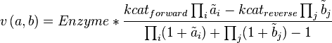
where variables with a tilde denote the normalised reactant concentrations $\tilde{a}$_i = [A_i] /K_mA and $\tilde{b}$_i = [B_i] /K_mB

General parameterisation

Strategies for Estimating Kinetic Parameter Values

Using Equilibrium Constant (K_eq) in the reversible Michaelis-Menten equation

Using the equilibrium constant in the reversible Michaelis-Menten reaction reduces the need to obtain or estimate Vmax_reverse parameter value, which is often not available in literature.

Using the Haldane relationship, the equilibrium constant (K_eq) can be written as:

${\color{Red}K_\mathrm{eq}} = [Enz]* \frac{Kcat_\mathrm{forward} * Km_\mathrm{product} }{Kcat_\mathrm{reverse} * Km_\mathrm{substrate}}$

Calculating the Equilibrium Constant (K_eq)

The equilibrium constant can be calculated from the ratio of the forward and reverse reaction rates as described in the above section, given that the values for these rates are known. Unfortunately, the information for these values are often difficult to find, especially for reverse reaction rates (Vmax_reverse).

As an alternative, the equlibrium constant, K_eq, can also be calculated from the Gibbs free energy of a reaction, ΔG_r, using the Van't Hoff isotherm equation:

$-ΔG^° = -RT ln K$

and by dividing both sides of the equation with RT, and later take the exponents of both sides, the K_eq can be calculated by this equation:

$K_\mathrm{eq} = exp \left ( \cfrac {-ΔG^{°'}}{RT} \right )$

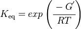
where;

Keq	Equilibrium constant
-ΔG°	Gibbs free energy change
R	Gas constant with a value of 8.31 JK-1mol-1
T	Temperature which is always expressed in kelvin

Brenda Add-on

For kinetic parameters describing enzymatic reactions, users have the option to further enrich the parameter value data by applying the BRENDA add-on. This add-on is an additional step in our DIPPER protocol after processing literature-derived parameter values. In this add-on protocol, background enzyme parameter values were retrieved from BRENDA according to a hierarchical rank. This hierarchical rank is based on two categories:- 1) the EC number of the enzyme of interest and 2) the modelled organism. Each of this category is the further broken down into several subcategories and is assigned to a weight value. The chosen weight from each category is then multiplied to give the total weight value for each dataset in the rank. Here, we name the dataset of each rank as an ‘EC case’. Since these are values retrieved from different organisms, different classes or subclasses and are more diverse than the literature values, the weights assigned to BRENDA values are lower than the ones assigned to values retrieved from literature specifically for the enzyme of interest, so that they will not dominate the final distribution, but rather give a more realistic picture of the plausible range of parameter values, and avoiding over-reliance on a limited set of experimental values. The (arbitrary) weights applied to the BRENDA data are summarised in Tables 1 and 2 respectively; before combining these values with the literature data, they are normalised, so that the total weight of all BRENDA data equals 10% of the sum of the weights of the literature values.

Table 1: Filtering categories for BRENDA data

Table 2: EC case hierarchy

How the DipperXBrenda function works

Both of these functions work by firstly filtering out the BRENDA datasets from ‘NaN’ values. To maintain significance of integrating these BRENDA data with literature values, only datasets with more than 50 values are considered. Then, these filtered or cleaned datasets are log-transformed into normal distributions. From there, the median and standard deviation is calculated. The exponents of these median and standard deviation are then calculated to obtain the mode and multiplicative factor for a log-normal distribution. Lastly, to normalise the weight of these BRENDA data, a normalising factor is calculated from a default 10% or from a user supplied percentage value, and the sum of weights that have been assigned to literature values. The outputs from the DipperXBrenda function are the mode, multiplicative factor, normalised weight and uncertainty type of ‘1’ for each of the dataset. These outputs are then compiled in a matrix that is ready to be merged with the literature values and will be used to calculate the overall log-normal distribution position (µ) and scale (σ) parameters. A summary of how both of these functions work is presented in Figure 1.

Fig. 1: Schematic representation of the DipperXBrenda function in the BRENDA add-on protocol. These functions require six datasets that are obtained from BRENDA, a vector of weights assigned to the literature values (Wo) and an optional percentage value (%) that will be used to normalise the weights assigned to the BRENDA data. Abbreviation used are as follows: Wo – vector of weights; % - percentage value; NaN – ‘not a number’; <50 – ‘less than 50 values’; DS- dataset; ‡ - predefined weights as described in the table; std – a MATLAB function to calculate standard deviation; median – a MATLAB function to calculate median; exp – a MATLAB function to calculate exponent, sum – a MATLAB function to calculate sum of values.

How to use the DipperXBrenda function

Step 1: Retrieve EC case datasets from BRENDA

In BRENDA, Km and turnover number (Kcat) values can be downloaded through its ‘Functional Parameter’ search query form. By inputting search terms as defined in table 1a, users are able to retrieve .csv files of each EC case (i.e. search terms ‘EC 1.2.3.*’ and ‘Escherichia coli’ would return values for EC case 1). Once the .csv files are ready, it can be imported into MATLAB either manually (by clicking on each respective *.csv file and select the value column) or using our importfile function (Supplementary). As the name suggests, this importfile function automatically imports the value column from each of the EC case text files. For example, this function can be used as follows:

This would import parameter values from text file ‘EC4_2_3_KmEcoli.csv’ that contains Km values with EC 4.2.3.* found in E. coli (EC case 1) and would assign the output to vector ‘DS1’.

Step 2: Calculate the mode, its uncertainty and assign weights for each of the EC cases.

Briefly, thes DipperXBrenda function work by first passing through six datasets (representing each EC case) as inputs to calculate the mode and its uncertainty. Then, weights are assigned to each EC case and normalised accordingly (Figure 1). The user would only need to run the function to use the BRENDA add-on as follows:

The first six arguments for both of the functions are the respective EC cases assigned to vectors (e.g. ‘DS1’, ‘DS2’) as described in Step 1. ‘Wo’ is a vector of literature-derived parameter value weights. The sum of the values in this vector is used as the benchmark to calculate the normalised weights based on a percentage value that the user can define in ‘Percent’. As a default, a value of 10% is assigned to this variable, which would mean that the total weight of all BRENDA data equals 10% of the sum of the weights of the literature values. The user can define different percentage values as follows:

The first line defines an example the ‘Wo’ vector. The second line shows how the user can define a percentage of 30%. The last line shows how the user can opt to not assign any values to the ‘Percent’ argument and in this case, the function will use the default 10%.

Step 3: Retrieve the resulting value matrix

The DipperXBrenda function would return an output matrix of four columns that corresponds to the mode, multiplicative factor (Mfact), normalised weight and uncertainty type respectively. For example:

For the uncertainty type column, ‘1’ is defined, as the uncertainty calculated for these BRENDA data is multiplicative. The units for Km and Kcat values from the DipperXBrenda function are mM and s-1 respectively. The output matrix ‘V1’ from this function can then be merged with literature-derived parameter values. Script 1 shows a full overview of the steps shown above. A detailed demonstration of how BRENDA add-on algorithm can be applied is described in case study 2. Figure 2 shows different parameter value distributions with and without integrating BRENDA data. The plots show that the distributions integrated with BRENDA data provided a more realistic range of parameter values without drastically adjusting the mode calculated from literature-derived values.

Script1: Step-by-step overview of how user can use DipperXBrenda function

Fig2: Comparison of parameter value distributions with and without BRENDA data. A) Probability distribution without considering additional background information from BRENDA; B) Probability distribution of Km_pulegone with the integration of BRENDA data where its total weight is 10% of the sum of weights from literature-derived parameter values, and C) Probability distribution of Km_pulegone with the integration of BRENDA data where its total weight is 30% of the sum of weights from literature-derived parameter values. Literature-derived parameter values are highlighted with dark blue lines and data from BRENDA is highlighted in light blue lines and asterisks. Comparison of plots A and B show that the spread of the parameter value distribution is bigger and Mode adjust accordingly when information from BRENDA is integrated. Meanwhile, comparison of plots of B and C show that the spread of the parameter values can be bigger when a higher weighting factor is assigned. Maximum and minimum value shown here encompasses 95.45% of confidence interval.

List of kinetic parameter values

Lists of values retrieved from published and unpublished sources for the kinetics of all the enzymes included in this study can be found here.

Abbreviations

List of abbreviations used in this study can be found here

Back to the main model page.

References

- ↑ Liebermeister, W. & Klipp, E. 2006. Bringing metabolic networks to life: convenience rate law and thermodynamics constraints.Theoretical Biology and Medical Modelling 3:41