Quantification of parameter uncertainty
Contents
- 1 Protocol for defining informative priors for ensemble modelling in systems biology
- 2 Overview of the protocol
- 3 Procedure
- 3.1 Step 1: Find and document parameter values
- 3.2 Step 2: Judge plausibility of values and assign weights
- 3.3 Step 3: Calculate the Mode and Spread of the probability distribution
- 3.4 Step 4: Calculate the location and scale parameters ( and ) of the log-normal distribution
- 3.5 Step 5: Account for thermodynamic consistency
- 4 References
Protocol for defining informative priors for ensemble modelling in systems biology
The quantification of parameter uncertainty is achieved by following a protocol [1] which aims to translate biological knowledge into informative probability distributions for every parameter, without the need for excessive mathematical and computational effort from the user. It assumes that a functioning kinetic model of the relevant biological system is already available and focuses on the procedures specific to the application of an ensemble modelling approach.
Overview of the protocol
The major protocol steps are the following:
- Collection and documentation of parameter information from the literature, databases and experiments.
- Plausibility assessment of each value collected from the literature using a standardized evidence weighting system. This includes assigning weights with regards to the quality, reliability and relevance of each experimental data point.
- Calculation of the Mode (most plausible value) and Spread (multiplicative standard deviation) using the weighted parameter data sets. These values are found using a function which calculates the weighted median and weighted standard deviation of the log transformed and normalised parameter values.
- Calculation of the location (
 ) and scale (
 ) parameters of the log-normal distribution based on the previously defined Mode and Spread.
 - If required, ensure the thermodynamic consistency of the model by creating multivariate distribution for interdependent parameters (e.g., the rates of forward and reverse reactions are connected via the equilibrium constant of the reaction, and must not be sampled independently).

Procedure
Step 1: Find and document parameter values
- Collect and document all available parameter values from literature, databases (e.g., BRENDA and BioNumbers) and experiments (hypothetical example displayed in Table 1).
- No values: If no values can be retrieved for a reaction occurring in a particular organism, broaden the search to include data from phylogenetically related organisms (the uncertainty should then be adjusted accordingly). When no values can be retrieved for a certain parameter, the broaden the search constraints; e.g., if the Michaelis–Menten constant,
 , for a particular substrate is unknown, it might be reasonable to retrieve all values from a database like BRENDA in order to determine the range of generally plausible values for this parameter. In cases where no parameter values are available, an indirect estimate is often possible, based on back-of-the-envelope calculations and fundamental biophysical constraints, which will have a larger uncertainty than a direct experimental measurement but will still be informative – situations where absolutely no information about a plausible parameter range is available will be extremely rare.
 - One value: If only a single experimental value will be available for a particular parameter, use this value as the Mode (most plausible value) of the probability distribution. Sometimes, an experimental error (e.g., a standard deviation) is reported for the value and can be used to estimate the Spread of plausible values; if this is not available an arbitrary multiplicative error can be assigned, based on a general knowledge of the reliability of a particular type of experimental technology. This information, of course, can be complemented using the previous strategy of retrieving related values from databases to optimise the estimate of the Spread of plausible values and avoid over-confident reliance on a single observation. Proceed to Step 4.
- More than one value: Whenever possible, it is important to collect as many experimental data with some implications for the range of plausible values, including those from a diverse range of methodologies, experimental conditions and biological sources. These will be pruned and weighted in the next step. Proceed to step 2.
- Document the reported experimental uncertainty (if available), in addition to the actual parameter value (Table 2).
- Uncertainty is reported in literature: Uncertainty is often reported as an (additive) standard deviation (SD) or a standard error of the mean (SEM). As the functions employed in the subsequent steps require standard deviations as inputs, reported standard errors should be converted to standard deviations for consistency. This can be achieved by multiplying by the square root of the sample size (n), as per the equation:
 . In cases where the sample size is not reported, a conservative value of n=3 can be assumed.
 - Uncertainty is not reported in literature:
- If the modeller is absolutely certain about a parameter value, the standard deviation can be set to zero. Although it is extremely rare that there is no uncertainty about a parameter at all, this option can be useful when designing the backbone topology of a model, prior to performing ensemble modelling, or when parts of the model are to be kept constant in all simulations.
- If the modeller has no information about the uncertainty of a reported parameter value, an arbitrary standard deviation can be assigned (e.g., the script provided for the next step assumes a default multiplicative standard deviation of 10% in such cases).
Note: Although uncertainty is usually reported in an additive form (x ± SD/SEM), theoretical biophysical considerations indicate that multiplicative errors often provide a better description about our actual uncertainty about experimental data in biology. For example, additive errors can imply that the confidence interval includes negative values. Thus, whenever possible, multiplicative standard deviations (Value */÷ SD) should be recorded. The script provided for the calculation of the probability distributions in Step 2 can handle both additive and multiplicative standard deviations. In order for the script to be able to distinguish between additive and multiplicative uncertainty, an extra column is added in the input file, where the uncertainty type is reported. This can be either 0 (additive standard deviation) or 1 (multiplicative standard deviation).
| Parameter Name | Reported values | Uncertainty | Sources |
|---|---|---|---|
 (μM) (μM)
|
0.5 | N/A | J. Poultry 2(3),2002 |
| 4.4 | ±0.2 (S.D.) | Quack Res. 4(6),1998 | |
| 10 | N/A | Antarctica Biol. 1(2),2004 | |
| 20 | ±1.5 (S.E.M.)(n=10) | Croc. Int. 10(3),2015 |
| Parameter Name | Reported values | Standard Deviation | Multiplicative/ Additive |
|---|---|---|---|
| (μM)
|
0.5 | 1.1 | Multiplicative (1) |
| 4.4 | 0.2 | Additive (0) | |
| 10 | 1.1 | Multiplicative (1) | |
| 20 | 4.7434 | Additive (0) |
Step 2: Judge plausibility of values and assign weights
When multiple parameter values are reported in the literature, assign appropriate weights according to their source. For the construction of larger models it can be helpful to use a standardized weighting scheme, to increase the internal consistency and reproducibility of the process. The weights will still be arbitrary, but they will consistently capture the modeller’s experience regarding the relative reliability of individual types of data. For example, standard weights can be assigned by answering a standard set of questions on the origin and properties of each parameter value:
- Is the value derived from an in vitro or in vivo experiment, and is this the same environment as in the experiment that will be simulated?
- Is the value derived from the modelled organism, from a phylogenetically related species, or from a completely unrelated system?
- Does the value concern the same enzyme (or protein / gene / receptor etc. depending on the case), a related class/superclass of enzyme, or a generic enzyme completely unrelated to the one used in the model?
- Are the experimental conditions (pH, temperature) the same, closely similar, or completely different from the ones simulated in the model?
According to the answer to each question, a standard partial weight can be assigned, and these weights can be multiplied to yield a total evidence weight for each experimental value (see Tables 3 and 4).
| Parameter values
|
Experimental Conditions
(In vivo, chicken, hexokinase, pH=7-7.5, 41.8±0.8oC) | |||
|---|---|---|---|---|
| In vivo/ in vitro | Organism | Enzyme | pH & Temperature | |
| 0.5 | In vitro | Chicken | Hexokinase | pH=8, 25oC |
| 4.4 | In vivo | Duck | Glucokinase | pH=7, 25oC |
| 10 | In vitro | Penguin | Hexokinase | pH=6.8, 40oC |
| 20 | In vitro | Crocodile | Glucokinase | pH=7, 41oC |
| Parameter values
|
Partial Weights | Total Weight | |||
|---|---|---|---|---|---|
| In vivo/ in vitro same as model? | Organism (same/ related/ unrelated) | Enzyme | Conditions (pH & temperature) | ||
| 0.5 | 1 (In vitro) | 4 (Same) | 4 (Same) | 4 (Same) | 64 |
| 4.4 | 2 (In vivo) | 2 (Related) | 2 (Related) | 1 (Unrelated) | 8 |
| 10 | 1 (In vitro) | 2 (Related) | 4 (Same) | 2 (Related) | 16 |
| 20 | 1 (In vitro) | 1 (Unrelated) | 2 (Related) | 4 (Same) | 8 |
Step 3: Calculate the Mode and Spread of the probability distribution
- Create a final input table which will include the parameter values, errors and weights that have been documented in Steps 1 and 2 (as shown in Table 5).
- Calculate the Mode and Spread of the probability distribution best describing our knowledge of the parameter values (Box 1) using the function CalcModeSpread.
Note: When no uncertainty estimate (e.g., standard deviation or standard error) is provided for an experimental parameter value (i.e., input for standard deviation is “NaN”), a multiplicative standard deviation of 10% (multiplicative factor 1.1) is automatically assigned to the parameter by the CalcModeSpread function, unless the uncertainty is explicitly set to zero. The standard assignment of the 10% multiplicative standard deviation is based on an extensive survey of reported error values in biology, but it remains arbitrary and can and should be modified by the user as appropriate.
| Parameter Name | Reported values | Standard Deviation | Total Weight | Multiplicative/ Additive |
|---|---|---|---|---|
| (μM)
|
0.5 | NaN | 64 | 1 |
| 4.4 | 0.2 | 8 | 0 | |
| 10 | NaN | 16 | 1 | |
| 20 | 4.7434 | 8 | 0 |
Box 1: How the CalcModeSpread function works
Using the summary table (Table 5) of the information gathered in Steps 1 and 2, the CalcModeSpread function calculates the Mode and Spread based on the weighted median and weighted standard deviation of the log-transformed experimental parameter values. The output of CalcModeSpread is used to create the final log-normal distribution in the next step, but its main use is to allow the model constructor an intuitive plausibility check of the translation process: the Mode represents the value most likely to be sampled, and the Spread by default represents a “multiplicative standard deviation”, the log-normal equivalent of the (additive) standard deviation of a normal distribution, i.e. it is calculated as a multiplicative error so that 68.27% of the sampled values will lie within the interval [Mode/Spread, Mode*Spread].
The CalcModeSpread function starts by calculating the weighted median and the weighted standard deviation of the log-transformed literature values, taking into account their uncertainty (e.g., standard deviation or multiplicative error) and reliability weighting specified in Step 2.
The calculations are based on the weighted median of the literature values rather than the (weighted) mean, as it is less likely to be biased by outliers and thus provide a more accurate description of the central tendency in the dataset. The algorithm implemented in CalcModeSpread defines the weighted median as the unique value מ with the property that exactly half of the probability weight is assigned to values in the interval [−∞, מ]. This approach, which expands earlier published algorithms for the calculation of weighted medians, circumvents the restriction that the weighted median can only be one of the values of the dataset (or the arithmetic mean of two adjacent values). The effects of different parameter weights and uncertainty on the weighted median are illustrated in Figure 2.

Once the weighted median and the weighted standard deviation have been calculated, they are exponentiated to yield the Mode and Spread (multiplicative standard deviation) of the final log-normal distribution.
Step 4: Calculate the location and scale parameters ( and ) of the log-normal distribution
The next part of the protocol is the calculation of the location () and scale () parameters of the log-normal distribution describing the parameter uncertainty (Box 2). The function CreateLogNormDist performs this surprisingly non-trivial transformation of the intuitive values of the Mode and Spread into the mathematically relevant properties of the log-normal distribution.
Box 2: How the CreateLogNormDist function works
The CreateLogNormDist function is based on the multiplicative symmetric property of the log-normal distribution. Log-normal distributions are symmetrical in the sense that a value that is x times larger than the most likely estimate (Mode) are just as plausible a value that is x times smaller. More specifically, the Mode of the distribution is the value  for which the condition
  is fulfilled for all positive real numbers
  , (where
  is the probability density function). By exploiting this property, the CreateLogNormDist function calculates an interval of values from the Mode and Spread provided. By default, 68.27% (or, more precisely
  , where
  ) of the sampled values should be in the confidence interval
 ![[x_{min}=\frac{Mode}{Spread},x_{max}=Mode\cdot Spread]](/wiki/images/math/6/c/a/6ca8529005411dc8c6527ad047d15064.png) . The default definition of the Spread can also be modified by the user, e.g. by requesting that 99% of values should be contained within the confidence interval – this flexibility can help in eliciting parameter estimates from experimentalist, especially in situations of high uncertainty. Based on the
. The default definition of the Spread can also be modified by the user, e.g. by requesting that 99% of values should be contained within the confidence interval – this flexibility can help in eliciting parameter estimates from experimentalist, especially in situations of high uncertainty. Based on the  and
and  values, a two-by-two system of the equations containing the cumulative distribution function (CDF) of the log-normal distribution and the Mode can be solved, in order to derive the location parameter μ and the scale parameter σ of the corresponding log-normal distribution:
where ![CDF(x)= \frac{1}{2}+\frac{1}{2} \mathrm{erf} \Big[\frac{lnx-\mu}{\sqrt{2}\sigma}\Big]](/wiki/images/math/c/e/d/ced4e79eb14d7986f52fb0ce29db3774.png) ,
,  is the error function and and are the lower and upper bounds of the confidence interval as defined before. By substituting these into the previous equation the final form of the system is obtained:
![\begin{cases}\frac{1}{2} \mathrm{erf} \Big[\frac{ln(Mode \cdot Spread)-\mu}{\sqrt{2}\sigma}\Big]-\frac{1}{2} \mathrm{erf} \Big[\frac{ln(\frac{Mode}{Spread})-\mu}{\sqrt{2}\sigma}\Big]=erf(\frac{1}{\sqrt{2}})\\
Mode=e^{\mu-\sigma^{2}}\end{cases}](/wiki/images/math/c/6/3/c6313a325574ba873f3e1bf3cc299dd1.png)
By algebraically solving this system of equations, the and parameters are obtained, and it is then easy to calculate any property in the distribution (e.g., the geometric mean and variance).
As in many cases log-normal distributions have long tails which may lead to sampling from a larger range of values than intended, the distributions can be truncated at a desired value. This is again best done in a multiplicative way. For instance, the modeler can decide how many times higher than the maximum value or lower than the minimum value among the experimental data points the sampling range should spread.
Step 5: Account for thermodynamic consistency
This step concerns parameters that cannot be independently sampled, because they are subject to thermodynamic constraints. In order to address the issue of thermodynamic consistency, joint probability distributions (multivariate distributions) can be employed for the interconnected parameters.
- Reversible Mass Action Reaction: Input the and the of all three initial (log-normal) distributions along with the number of parameter samples that should be generated in the function Multivariate3param. The function then generates the requested number of parameter triplets, by using the strategy detailed in Box 3.
- Enzymatic Reactions: For the 5-parameter Michaelis−Menten kinetics, input the μ and the σ of all five initial distributions as derived in Steps 1–4 of the protocol, along with the number of parameter samples that should be generated the Multivariate5param function. The function then generates the requested number of parameter sets by using the principles described above, by using the strategy described in Box 4. This strategy can be expanded to even more complex cases which would require more than five parameters (e.g., Bi–Bi, Uni–Bi, Ter–Ter mechanisms etc.), by using the internal mass action kinetic reactions to define the correlations of the external Michaelis−Menten parameters.
- Futile Cycles: Finally, it is possible that substrate (futile) cycles may be a part of a biological model. For each closed loop in the metabolic pathways, the total Gibbs free energy change (
 ) has to be zero as an additional thermodynamic constraint. This means that the equilibrium constants of the reactions involved in the cycle will need to additionally comply with the constraint
  . In order to address this aspect of the system, e.g. for a three reaction loop, correlate the parameters for two of the reactions independently as described above, and calculate the
  of the third reaction from the Gibbs energy equation (
 ). Finally, pass the values calculated for
  on the internal system of equations (Michaelis-Menten, mass action etc.) of the third reaction and thus create the additional correlations.
Box 3: Thermodynamic consistency in a reversible mass action reaction
In a simple reversible mass action reaction, three interconnected parameters are involved (the association rate ( ), the dissociation rate (
 ), and the equilibrium constant (
 )) (Figure 3). The three values are connected by the equation
  , and the plausible combinations of rate constants will depend on our uncertainty about the equilibrium constant (i.e., if we have very precise information about the position of the equilibrium, only a very limited range of combinations will be consistent with this thermodynamic information, while in the absence of thermodynamic information, any combination of rate constants is allowed). Of course, in principle, each of the three parameters has equal status, and the multivariate distribution for sampling can be constructed in three different ways, each expressing the dependency between two sampled parameters in terms of the third.
 , ) a bivariate system of distributions is created. When the two marginal distributions are non-correlated the generated points which represent parameter pairs, form a circle. When is exactly known, (the parameters and are tightly correlated through the ) the points form a straight line. Finally, if is approximately known (a distribution of values for exists) the resulting points of the bivariate system form an ellipse. The thickness and orientation of the ellipse depend on the magnitude of the correlation between the two marginal distributions and on the degree of uncertainty on the values of , and . This case represents the realistic scenario when modelling, as usually the parameter values are approximately known. The first case (no correlation) does not respect thermodynamic consistency and is therefore undesirable. The second case, although taking into account the dependency of the two parameters, is in most cases unrealistic since the value of a parameter is rarely exactly known.
For instance, the two marginal distributions can be and (= ), where is dependent on the values of and . An overview of the steps followed is outlined in Figure 4. In order to decide which parameter will be the dependent one, the geometric coefficient of variation (GCV) is calculated for each parameter (
 ), and the parameter with the largest geometric coefficient of variation is set as the dependent variable (this is the parameter with the largest uncertainty, and sampling from the multivariate distribution will result in an increase of variance for the dependent parameter). The calculation of the dependent parameter is enabled by another property of the log-normal distributions: any product of two independent log-normal random variables is also log-normally distributed. Therefore, for the two log-normal distributions
 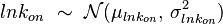 and
and 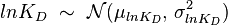 , their product will be the log-normal distribution
  and its location and scale parameters will be
  ,
,  . A similar argument applies for the quotient of two log-normal distributions, although in this case the parameter will be derived by the formula
  . The formula for the calculation of the parameter does not change. Note that while log-normal distributions are sometimes counterintuitive to use, this useful and unique property alone would be sufficient justification for using them as often as possible in the definition of biologically informative priors, in preference over uniform or standard normal distributions.

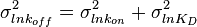
It is then very easy to transform the two marginal distributions and to normal ones, via the natural logarithm. The problem can therefore be reduced to the case of a multivariate normal distribution with the following probability density function:
![f(x,y) =
\frac{1}{2 \pi \sigma_X \sigma_Y \sqrt{1-\rho^2}}
\exp\left(
-\frac{1}{2(1-\rho^2)}\left[
\frac{(x-\mu_X)^2}{\sigma_X^2} +
\frac{(y-\mu_Y)^2}{\sigma_Y^2} -
\frac{2\rho(x-\mu_X)(y-\mu_Y)}{\sigma_X \sigma_Y}
\right]
\right)](/wiki/images/math/9/e/4/9e402fdfb11e31cee2b495bdce33d97d.png)
where  is the correlation between
  and
and  and
and  and
and  . In this case,
  (covariance matrix).
The parameters are assumed to be independent if = 0, so there is no correlation between them. Otherwise, the resulting bivariate iso-density loci plotted in the x,y-plane are ellipses. As the correlation parameter increases, these loci appear to be squeezed to the following line:
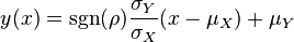
In this way, thermodynamically consistent triplets of , and parameters can be sampled, which can then be used for the model simulations.
Note: The required parameter values are obtained by generating samples from the multivariate normal distribution and then exponentiating the results. In order to avoid errors that are introduced to the correlation matrix during the exponentiation, the matlab function "Multivariate Log-normal Simulation with Correlation" (MVLOGNRAND) is used, which makes up for these errors.
Box 4: Thermodynamic consistency in a 5-parameter Michaelis–Menten enzymatic reaction
The same strategy applied for the three parameter mass action kinetics (Box 3), can be expanded to slightly more complex reaction schemes, such as reversible enzymatic reactions. The simplest case in this category would be a reaction where a single substrate is transformed to a single product (Uni–Uni reaction) as per:

This reaction is usually described by Michaelis−Menten kinetics, where the parameters  and
and  are linked with the through the Haldane equation:
  . In this case, the dependencies and correlations of the parameters are defined in two stages (Figure 5). In Stage 1, the parameter with the largest geometric coefficient of variation is set as the dependent one (as in the 3 parameter case) and is recalculated from the independent parameters through the Haldane equation. In Stage 2, the internal mass action kinetics parameters
  , derived by using the King−Altman method, are used to define the correlations between the observed (external) parameters
 and . The internal parameters can be derived from the external ones manually or, for more complex reactions, algorithms and online tools that automate the process can be employed.
For example, the transformation equations for the Uni–Uni reaction are the following:

The marginal distributions in this case are for the parameters  and , and the mass action kinetics parameters ,
  and
and  are used to calculate the covariance matrix and thus define the correlations within the system. The mathematical properties are similar to the ones employed in the three parameter case, being based on the properties of products and quotients of log-normal distributions and additionally using the Fenton−Wilkinson approximation for the addition of two independent log-normal distributions:
![\begin{align}
\sigma^2_Z &= \ln\!\left[ \frac{\sum e^{2\mu_j+\sigma_j^2}(e^{\sigma_j^2}-1)}{(\sum e^{\mu_j+\sigma_j^2/2})^2} + 1\right] \\
\mu_Z &= \ln\!\left[ \sum e^{\mu_j+\sigma_j^2/2} \right] - \frac{\sigma^2_Z}{2}
\end{align}](/wiki/images/math/7/9/d/79d0640c787886e5485958f8683b417c.png)
where  and
and  are the parameters of the initial log-normal distributions and
  and
and  are the parameters of the log-normal distribution representing their sum.
