Quantification of parameter uncertainty

Design of probability distributions

Example of defining the log-normal distribution by using the confidence interval factor. The red line is defining a log-normal distribution with $\mu$=1.5653 and $\sigma$=0.4231. The mode is equal to 4 is represented by the blue line, the mean is equal to 5.2 and is represented by the green line and the median is equal to 4.8 and is represented by the yellow line. The grey area highlights the range between 1.6 and 10 within which lie 95.45% of the values, calculated by choosing a confidence interval factor of 2.5. The value 10 and the value 1.6 have equal probability of being sampled (f(4*2.5) =f(4/2.5)=0.2066).

In order to create the probability distributions, the location and scale parameters $\mu$ and $\sigma$ were required. These can be easily calculated from the mean and standard deviation of the available sample data. However in many cases, there were very little or no reported values for a parameter, or there was a minimum and maximum reported value. It was therefore necessary to come up with an alternative way to derive them which at the same time would be understandable to experimentalists, without demanding complicated mathematical terms and calculations.

In order to achieve this, the mode of the log-normal distribution (global maximum) and its symmetric properties were employed. Log-normal distributions are symmetrical in the sense that values that are $x$ times larger than the most likely estimate, are just as plausible as values that are $x$ times smaller. More specifically, the mode of the distribution is the value $x_0$ for which the condition 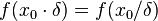$f(x_0 \cdot \delta)=f(x_0 / \delta)$ for all real numbers $\delta$, (where $f$ is the probability density function) is fulfilled. Hence, the user has to decide on a most plausible value for each parameter, which is set as the mode (global maximum) of the corresponding distribution (Probability Density Function or PDF), and on a range within which lie 95.45% of the values. The latter is linked to the mode via a multiplicative factor, which we call "Confidence Interval Factor". If the mode is multiplied or divided by the CI factor, the range within which 95.45% of the values are found is calculated. For instance, if the most plausible value for a parameter is $X$ and the confidence interval multiplicative factor is $y$, then the mode of the distribution is set as $X$ the range where 95.45% of the plausible values are found is $[\frac{X}{y},X\cdot y]$.

Based on these values, a two-by-two system of the equations containing the cumulative distribution function (CDF) and the mode is solved, in order to derive the location parameter $\mu$ and the scale parameter $\sigma$ of the corresponding log-normal distribution. The equations are the following:

$\begin{cases}CDF(x_{max})-CDF(x_{min})=0.9545\\ Mode=e^{\mu-\sigma^{2}}\end{cases}$

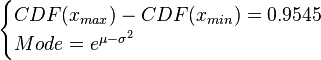
where $CDF= \frac{1}{2}+\frac{1}{2} \mathrm{erf} \Big[\frac{lnx-\mu}{\sqrt{2}\sigma}\Big]$ and $x_{min}$ and $x_{max}$ are the lower and upper bounds of the confidence interval. By substituting these into the previous equation the final form of the system is obtained:

$\begin{cases}\frac{1}{2} \mathrm{erf} \Big[\frac{lnx_{max}-\mu}{\sqrt{2}\sigma}\Big]-\frac{1}{2} \mathrm{erf} \Big[\frac{lnx_{min}-\mu}{\sqrt{2}\sigma}\Big]=0.9545\\ Mode=e^{\mu-\sigma^{2}}\end{cases}$

In this way, the $\mu$ and $\sigma$ parameters are obtained and from them it is easy to calculate any property in the distribution (i.e. geometric mean, variance etc.)

Parameter dependency and thermodynamic consistency

In some cases, parameters cannot be chosen separately either because they are statistically dependent, subject to thermodynamic constraints or depend on another common parameter. Therefore, thermodynamic consistency is also an important factor that needs to be considered to decide if the combinations of parameters are plausible. For instance, a very common occurrence in biological systems are forward and backward reactions. The source of dependency is the equilibrium constant, which denotes the relationship between the kinetic parameters for the "on" and "off" components of the reaction. Let’s assume a reaction that is known to have an equilibrium constant very close to 1, i.e. its standard Gibbs free energy $\Delta G^o$ = 0. There is not much information about the rate of the reaction, so each of the two parameters is sampled from a very broad distribution. If the additional thermodynamic information is not taken into account, there will often be cases where values will be sampled from the "fast" end of the spectrum for the forward reaction rate, and from the "slow" end for the backward rate (or vice versa). Thus, inconsistent pairs of the two parameters will be generated. In this case, thermodynamic consistency requires that we discard such samples and only keep those where the two reaction rates are very similar (how similar will in turn depend on our uncertainty about the equilibrium constant).

In order to address this problem we are employing a joint probability distribution (multivariate distribution) for the two parameters (i.e. $k_{on}$ and $k_{off}$), in order to ensure that each of the generated values for both of them are constrained within a specified range. Additionally, this approach ensures that their dependency on each other and on the equilibrium constant $K_{D}$ is taken into account and quantified appropriately.

For instance, if the two marginal distributions are $k_{on}$ and $k_{on}\cdot K_D$ (=$k_{off}$), $k_{off}$ is dependent on the values of $k_{on}$ and $K_D$. The parameter with the largest geometric coefficient of variation (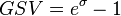$GSV=e^{\sigma}-1$) is usually set as the dependent one. Any product of two log-normal random variables is also log-normally distributed. 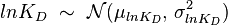Therefore, for the two log-normal distributions $ln k_{on}\ \sim\ \mathcal{N}(\mu_{ln k_{on}},\, \sigma^{2}_{ln k_{on}})$ and $ln K_D\ \sim\ \mathcal{N}(\mu_{ln K_D},\, \sigma^{2}_{ln K_D})$, their product $k_{off}$ will be the log-normal distribution $ln k_{off}\ \sim\ \mathcal{N}(\mu_{ln k_{on}}+\mu_{ln K_D},\, \sigma^{2}_{ln k_{on}}+\sigma^{2}_{ln K_D})$ and its parameters will be $\mu_{ln k_{off}}=\mu_{ln k_{on}}+\mu_{ln K_D}$, $\sigma^{2}_{ln k_{off}}=\sigma^{2}_{ln k_{on}}+\sigma^{2}_{ln K_D}$.

A similar strategy applies for the quotient of two log-normal distributions, although in this case the parameter $\mu$ will be derived by the formula $\mu_{quotient}=\mu_{dividend}-\mu_{divisor}$. The formula for the calculation of the parameter $\sigma$ does not change.

Thus, it becomes easy to transform the two marginal distributions $k_{on}$ and $k_{off}$ to normal ones, through the natural logarithm. The problem can therefore be reduced to the case of a multivariate normal distribution generated by the formula

Failed to parse (syntax error): f(x,y)= \frac{1}{2 \pi \sigma_X \sigma_Y \sqrt{1-\rho^2}} \exp\left( -\frac{1}{2(1-\rho^2)}\left[ \frac{(x-\mu_X)^2}{\sigma_X^2} + \frac{(y-\mu_Y)^2}{\sigma_Y^2} - \frac{2\rho(x-\mu_X)(y-\mu_Y)}{\sigma_X \sigma_Y}\right] \right)\\

where $\rho$ is the correlation between $X (=k_{on})$ and $Y (=k_{off})$ and $\sigma_X > 0$ and $\sigma_Y > 0$. In this case, 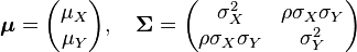$\boldsymbol\mu = \begin{pmatrix} \mu_X \\ \mu_Y \end{pmatrix}, \quad \boldsymbol\Sigma = \begin{pmatrix} \sigma_X^2 & \rho \sigma_X \sigma_Y \\ \rho \sigma_X \sigma_Y & \sigma_Y^2 \end{pmatrix}$ (covariance matrix).

The parameters are assumed to be independent if \rho = 0, so there is no correlation between them. Otherwise, the resulting bivariate iso-density loci plotted in the x,y-plane are ellipses (Figure 4a). As the correlation parameter \rho increases, these loci appear to be squeezed to the following line:

$y(x)= \mathop{\rm sgn} (\rho)\frac{\sigma_Y}{\sigma_X} (x- \mu_X) + \mu_Y$

Sampling strategy for maintaining thermodynamic consistency of parameter sets. In order to ensure the thermodynamic feasibility of a parameter combination in the case of interconnected parameters (i.e. forward and backward reaction, k_{on}, k_{off}) a bivariate system of distributions is created. When the two marginal distributions are non-correlated the generated points which represent parameter pairs, form a circle. When KD is exactly known, (the parameters k_{on} and k_{off} are tightly correlated through the K_D) the points form a straight line. Finally, if K_D is approximately known (a distribution of values for K_D exists) the resulting points of the bivariate system form an ellipse. The thickness and orientation of the ellipse depend on the magnitude of the correlation between the two marginal distributions and on the degree of uncertainty on the values of k_{on}, k_{off} and K_D. This case represents the realistic scenario when modelling, as usually the parameter values are approximately known. The first case (no correlation) does not respect thermodynamic consistency and is therefore undesirable. The second case, although taking into account the dependency of the two parameters, is in most cases unrealistic since the value of a parameter is rarely exactly known.

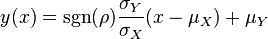
The required parameter values are obtained by generating samples from the multivariate normal distribution and then exponentiating the results. In order to avoid errors that are introduced to the correlation matrix during the exponentiation, a matlab function called Multivariate Lognormal Simulation with Correlation (MVLOGNRAND) is used, which makes up for these errors.