Difference between revisions of "Binding of R2 to A"
(→Parameters) |
(→Parameters) |
||
| (47 intermediate revisions by the same user not shown) | |||
| Line 8: | Line 8: | ||
==Chemical equation== | ==Chemical equation== | ||
| − | <center><math>A + R_{2} \rightleftharpoons | + | <center><math>A + R_{2} \rightleftharpoons AR_{2}</math></center> |
== Rate equation == | == Rate equation == | ||
| − | <center><math> r= \frac{k^{-}_{3}}{K_{d3}}\cdot [A]\cdot [R_{2}] - k^{-}_{3}\cdot [ | + | <center><math> r= \frac{k^{-}_{3}}{K_{d3}}\cdot [A]\cdot [R_{2}] - k^{-}_{3}\cdot [AR_{2}]</math></center> |
== Parameters == | == Parameters == | ||
| Line 31: | Line 31: | ||
|- | |- | ||
|<math>K_{d3}</math> | |<math>K_{d3}</math> | ||
| − | |<math>10^{ | + | |<math>10^{4}-10^{6} </math> <ref name="Saliha2011"></ref> |
| <math>nM</math> | | <math>nM</math> | ||
| − | | <math>0.083 nM^{-1} s^{-1}</math> | + | | <math>0.083 nM^{-1} s^{-1}</math> |
| − | |||
| − | (Bistability range: <math>0.083-0.12 nM^{-1} s^{-1}</math>) | + | <math>(4.98 nM^{-1} min^{-1})</math> |
| − | |According to the Ozbabacan et al. association constants for transient protein protein interactions lie in the millimolar or micromolar range. | + | |
| + | Range tested: <math>10^{-7}-10^{-1} nM^{-1} s^{-1}</math> | ||
| + | |||
| + | <math>(6 \cdot 10^{-6}-6 nM^{-1} min^{-1})</math> | ||
| + | |||
| + | Bistability range: <math>0.083-0.12 nM^{-1} s^{-1}</math> | ||
| + | |||
| + | (<math>4.98-7.2 nM^{-1} min^{-1}</math>) | ||
| + | |According to the Ozbabacan et al. association constants for transient protein protein interactions lie in the millimolar or micromolar range. (<math> 10^{3} (or 10^{4})-10^{6}nM</math>) | ||
[[Image:Kd3-text.png|center|thumb|350px|Ozbabacan et al. 2011<ref name="Saliha2011"></ref>]] | [[Image:Kd3-text.png|center|thumb|350px|Ozbabacan et al. 2011<ref name="Saliha2011"></ref>]] | ||
|- | |- | ||
|<math>k^{-}_{3}</math> | |<math>k^{-}_{3}</math> | ||
| − | |<math> | + | |<math>38.3-4.46 \cdot 10^{6}</math> <ref name="Janin1997"> [http://onlinelibrary.wiley.com/doi/10.1002/(SICI)1097-0134(199706)28:2%3C153::AID-PROT4%3E3.0.CO;2-G/epdf Janin, Joel. ''The kinetics of protein-protein recognition.'' Proteins-Structure Function and Bioinformatics (1997): 153-161.]</ref> <ref name="Northrup1992"> [http://www.pnas.org/content/89/8/3338.full.pdf Northrup S.H. and Erickson H.P. ''Kinetics of protein-protein association explained by Brownian dynamics computer simulation.''PNAS 1992;89(8),3338-3342]</ref> |
|<math>min^{-1}</math> | |<math>min^{-1}</math> | ||
| − | | <math>630 s^{-1}</math> | + | | <math>630 s^{-1} (37800 min^{-1})</math> |
| − | + | Range tested: <math>0- 10^{3} s^{-1}</math> | |
| + | |||
| + | <math>(0-6 \cdot 10^{4} min^{-1})</math> | ||
| + | |||
| + | Bistability range: <math>460-630 s^{-1}</math> | ||
| − | + | <math>(27600-37800 min^{-1})</math> | |
| − | |According to Northrup et al. the | + | |According to Northrup et al. the association rate of protein-protein bond formations occur in the order of <math>10^{6} M^{-1}s^{-1}</math>. |
[[Image:K3-text.png|center|thumb|350px|Northrup et al. 1992<ref name="Northrup1992"></ref>]] | [[Image:K3-text.png|center|thumb|350px|Northrup et al. 1992<ref name="Northrup1992"></ref>]] | ||
| + | |||
| + | These values are also supported by Ozbabacan et al. who claim that association rates are usually in the range <math>10^5-10^6 M^{-1}s^{-1}</math> (<math>0.006-0.06 nM^{-1}min^{-1}</math>). | ||
| + | [[Image:K3-text2.png|center|thumb|350px|Ozbabacan et al. 2011<ref name="Saliha2011"></ref>]] | ||
| + | |||
| + | Therefore, these values are used to generate the probability distribution for <math>k_{on3}</math> as described in the following section. | ||
| + | |||
| + | Afterwards, the log-normal distribution for the dissociation rate of the ScbR-ScbA binding (<math>k^{-}_{3}</math>) is derived from the distributions of <math>K_{d3}</math> and <math>k_{on3}</math>. | ||
|} | |} | ||
==Parameters with uncertainty== | ==Parameters with uncertainty== | ||
| − | Since the values we are using for this parameter correspond to generic association constant values of a wide range of protein-protein interactions and not specifically to GBL or related systems, we wish to explore the whole range of values and investigate the conditions under which the ScbR-ScbA complex formation would be feasible. Therefore, | + | Since the values we are using for this parameter correspond to generic association constant values of a wide range of protein-protein interactions and not specifically to GBL or related systems, we wish to explore the whole range of values and investigate the conditions under which the ScbR-ScbA complex formation would be feasible. Therefore, by assigning the appropriate weights to the parameter values and using the method described [[Quantification of parameter uncertainty#Design of probability distributions|'''here''']], the appropriate probability distributions were designed. The mode of the log-normal distribution for <math>K_{d3}</math> is <math> 9.95 \cdot 10^{4} nM </math> and the Spread to <math> 10 </math>. Thus, the range where 68.27% of the values are found is between <math> 9.93 \cdot 10^{3} nM </math> and <math> 9.97 \cdot 10^{5} nM </math>. |
| + | |||
| + | Similarly, by following the same reasoning, the mode of the log-normal distribution for <math>k_{on3}</math> is set to <math>0.018 nM^{-1} min^{-1}</math> and the Spread to <math>3.17</math>. This means that the range where 68.27% of the values are found is between <math> 0.0059 nM^{-1} min^{-1}</math> and <math>0.06 nM^{-1} min^{-1}</math>. | ||
| + | |||
| + | Since the two parameters are interdependent, thermodynamic consistency also needs to be taken into account. This is achieved by creating a bivariate system as described [[Quantification of parameter uncertainty#Parameter dependency and thermodynamic consistency|'''here''']]. Since no information was retrieved for <math>k^{-}_{3}</math> and therefore is the parameter with the largest geometric coefficient of variation, this is set as the dependent parameter as per: <math>k^{-}_{3}=k_{on3} \cdot K_{d3}</math>. The location and scale parameters of <math>k^{-}_{3}</math> (μ=9.9423 and σ=1.5503) were calculated from those of <math>K_{d3}</math> and <math>k_{on3}</math>. | ||
| − | + | The probability distributions for the three parameters, adjusted accordingly in order to reflect the above values, are the following: | |
| − | + | [[Image:KD3u.png|500px]] [[Image:Kon3u.png|500px]] [[Image:K3u.png|500px]] | |
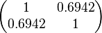
| − | + | The correlation matrix which is necessary to define the relationship between the two marginal distributions (<math>k_{d3}</math>,<math>k^{-}_{3}</math>) of the bivariate system is derived by employing random values generated by the two distributions. | |
| − | The | + | The parameter information of the distributions of the multivariate system is: |
{|class="wikitable" | {|class="wikitable" | ||
! Parameter | ! Parameter | ||
| + | ! Mode | ||
| + | ! Spread | ||
! μ | ! μ | ||
! σ | ! σ | ||
| + | ! Correlation matrix | ||
| + | |- | ||
| + | |<math>k_{on3}</math> | ||
| + | |<math>0.0188</math> | ||
| + | |<math>3.17</math> | ||
| + | |<math>-3.2497</math> | ||
| + | |<math>0.84825</math> | ||
| + | |N/A | ||
|- | |- | ||
|<math>K_{d3}</math> | |<math>K_{d3}</math> | ||
| − | |<math> | + | |<math>99547</math> |
| − | |<math>0. | + | |<math>10.02</math> |
| + | |<math>13.192</math> | ||
| + | |<math>1.2977</math> | ||
| + | |rowspan="2"|<math>\begin{pmatrix} 1 & 0.6942 \\ | ||
| + | 0.6942 & 1 \end{pmatrix}</math> | ||
|- | |- | ||
|<math>k^{-}_{3}</math> | |<math>k^{-}_{3}</math> | ||
| − | |<math> | + | |N/A |
| − | |<math> | + | |N/A |
| + | |<math>9.9423</math> | ||
| + | |<math>1.5503</math> | ||
|} | |} | ||
| + | |||
| + | The multivariate system of the normal distributions (<math>ln(k_{d3})</math> and <math>ln(k^{-}_{3})</math>) and the resulting samples of values are presented in the following figure: | ||
| + | |||
| + | [[Image:Multidist3.png|500px]] | ||
| + | |||
| + | In this way, a system of distributions is created where each distribution is described and constrained by the other two. Therefore, the parameters will be sampled by the two marginal distributions in a way consistent with our beliefs and with the relevant thermodynamic constraints. | ||
==References== | ==References== | ||
<references/> | <references/> | ||
Latest revision as of 18:59, 2 January 2018
The ScbR homo-dimer (R2) forms a complex with ScbA (A).


Contents
Chemical equation
Rate equation
![r= \frac{k^{-}_{3}}{K_{d3}}\cdot [A]\cdot [R_{2}] - k^{-}_{3}\cdot [AR_{2}]](/wiki/images/math/c/0/6/c06b35d93c94434b80e84d47aeff0944.png)
Parameters
The parameters of this reaction are the dissociation constant for binding of ScbR to ScbA ( ) and the dissociation rate for binding of ScbR to ScbA (
 ). Since there is no concrete evidence of the existence of the ScbA-ScbR complex so far, it is possible that the interaction between the two proteins is unstable/ transient and therefore the parameter values reflect this belief. The values of such complexes according to the literature [1] , lie in the millimolar or micromolar scale.

| Name | Value | Units | Value in previous GBL model [3] | Remarks-Reference |
|---|---|---|---|---|
|
|
 [1] [1]
|

|
Range tested:
Bistability range: ( |
According to the Ozbabacan et al. association constants for transient protein protein interactions lie in the millimolar or micromolar range. ( ) )
 Ozbabacan et al. 2011[1] |
|
|
 [4] [5] [4] [5]
|

|
Range tested:
Bistability range:
|
According to Northrup et al. the association rate of protein-protein bond formations occur in the order of  . .
 Northrup et al. 1992[5] These values are also supported by Ozbabacan et al. who claim that association rates are usually in the range  Ozbabacan et al. 2011[1] Therefore, these values are used to generate the probability distribution for Afterwards, the log-normal distribution for the dissociation rate of the ScbR-ScbA binding ( |
 )
)

 (
( ).
).
Parameters with uncertainty
Since the values we are using for this parameter correspond to generic association constant values of a wide range of protein-protein interactions and not specifically to GBL or related systems, we wish to explore the whole range of values and investigate the conditions under which the ScbR-ScbA complex formation would be feasible. Therefore, by assigning the appropriate weights to the parameter values and using the method described here, the appropriate probability distributions were designed. The mode of the log-normal distribution for is  and the Spread to
  . Thus, the range where 68.27% of the values are found is between
  and
and  .
.
Similarly, by following the same reasoning, the mode of the log-normal distribution for  is set to
  and the Spread to
  . This means that the range where 68.27% of the values are found is between
  and
and  .
.
Since the two parameters are interdependent, thermodynamic consistency also needs to be taken into account. This is achieved by creating a bivariate system as described here. Since no information was retrieved for and therefore is the parameter with the largest geometric coefficient of variation, this is set as the dependent parameter as per:  . The location and scale parameters of (μ=9.9423 and σ=1.5503) were calculated from those of and .
The probability distributions for the three parameters, adjusted accordingly in order to reflect the above values, are the following:


The correlation matrix which is necessary to define the relationship between the two marginal distributions ( ,) of the bivariate system is derived by employing random values generated by the two distributions.
The parameter information of the distributions of the multivariate system is:
| Parameter | Mode | Spread | μ | σ | Correlation matrix |
|---|---|---|---|---|---|
|
|

|
|

|

|
N/A |
|
|

|

|

|

|
|
|
|
N/A | N/A | 
|

|
The multivariate system of the normal distributions ( and
and  ) and the resulting samples of values are presented in the following figure:

In this way, a system of distributions is created where each distribution is described and constrained by the other two. Therefore, the parameters will be sampled by the two marginal distributions in a way consistent with our beliefs and with the relevant thermodynamic constraints.
References
- ↑ 1.0 1.1 1.2 1.3 1.4 Saliha Ece Acuner Ozbabacan, Hatice Billur Engin, Attila Gursoy, and Ozlem Keskin. Transient protein–protein interactions. Protein Engineering, Design and Selection first published online June 15, 2011
- ↑ Perkins J. R., Diboun I., Dessailly B. H., Lees J. G., Orengo C. Transient Protein-Protein Interactions: Structural, Functional, and Network Properties. Structure, 2010;18:10, p. 1233-1243
- ↑ S. Mehra, S. Charaniya, E. Takano, and W.-S. Hu. A bistable gene switch for antibiotic biosynthesis: The butyrolactone regulon in streptomyces coelicolor. PLoS ONE, 3(7), 2008.
- ↑ Janin, Joel. The kinetics of protein-protein recognition. Proteins-Structure Function and Bioinformatics (1997): 153-161.
- ↑ 5.0 5.1 Northrup S.H. and Erickson H.P. Kinetics of protein-protein association explained by Brownian dynamics computer simulation.PNAS 1992;89(8),3338-3342